Usage

Basic Usage

compute_melt_pool accepts a pandas.DataFrame of process and material parameters and returns the same DataFrame with melt pool dimensions appended as new columns.

import pandas as pd
from eagar_tsai import compute_melt_pool

df = pd.read_excel("my_parameters.xlsx")

# Rename columns to match required names if needed
df = df.rename(columns={
    "Velocity_m/s": "velocity_m_s",
    "Power": "power_w",
    "Beam_diameter_m": "beam_diameter_m",
    "Absorptivity": "absorptivity",
    "T_liquidus": "liquidus_temperature_k",
    "thermal_cond_liq": "thermal_conductivity_w_mk",
    "Density_kg/m3": "density_kg_m3",
    "Cp_J/kg": "specific_heat_j_kgk",
})

result = compute_melt_pool(df, workers=4, chunk_size=10)
result.to_csv("melt_pool_results.csv", index=False)

Input Data Format

compute_melt_pool accepts a pandas.DataFrame with the following columns:

Column	Unit	Description
velocity_m_s	m/s	Scan velocity
power_w	W	Laser power
beam_diameter_m	m	Beam diameter (2σ)
absorptivity	—	Absorptivity (0, 1]
liquidus_temperature_k	K	Liquidus temperature
thermal_conductivity_w_mk	W/(m·K)	Thermal conductivity at liquidus
density_kg_m3	kg/m³	Density
specific_heat_j_kgk	J/(kg·K)	Specific heat at liquidus

Output Columns

The result DataFrame contains all input columns plus:

Column	Unit	Description
melt_length	m	Melt pool length
melt_width	m	Melt pool width (full, 2× half-width)
melt_depth	m	Melt pool depth
melt_length_um	µm	Melt pool length
melt_width_um	µm	Melt pool width
melt_depth_um	µm	Melt pool depth
peak_temperature	K	Peak temperature in domain
min_temperature	K	Minimum temperature in domain

Single-Point Computation

For a single parameter set, use compute_single_point directly. It returns a MeltPoolResult that always includes the full TemperatureField.

from eagar_tsai import BeamParameters, MaterialProperties, SimulationDomain, compute_single_point

beam = BeamParameters(
    beam_diameter=100e-6,         # m
    power=200.0,                  # W
    velocity=0.5,                 # m/s
    absorptivity=0.35,            # —
)

material = MaterialProperties(
    liquidus_temperature=1700.0,  # K
    thermal_conductivity=30.0,    # W/(m·K)
    density=7800.0,               # kg/m³
    specific_heat=700.0,          # J/(kg·K)
)

domain = SimulationDomain(
    x_length_um=1200.0,           # µm
    y_length_um=1200.0,           # µm
    z_depth_um=1000.0,            # µm
    spatial_resolution_um=1.0,    # µm
)

result = compute_single_point(beam, material, domain)

print(f"Length: {result.length_um:.1f} µm")
print(f"Width:  {result.width_um:.1f} µm")
print(f"Depth:  {result.depth_um:.1f} µm")

Temperature Field Visualization

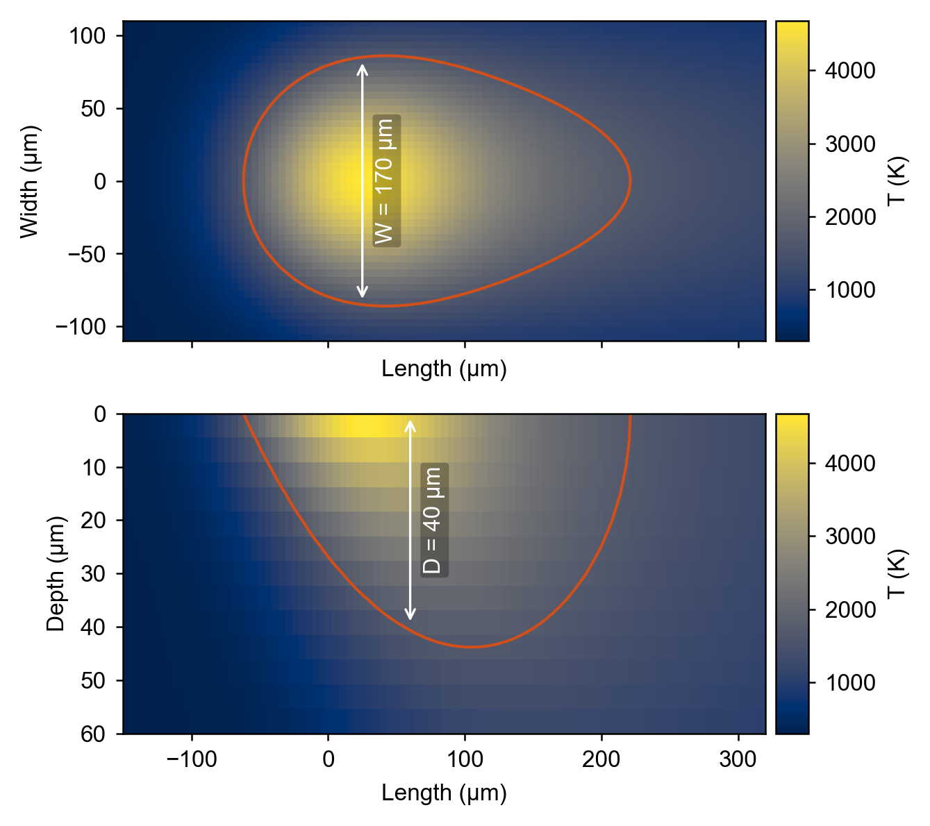
compute_single_point returns a MeltPoolResult that always includes a TemperatureField with direct access to the raw arrays and a built-in plot method.

from eagar_tsai import BeamParameters, MaterialProperties, SimulationDomain, compute_single_point

beam = BeamParameters(
        beam_diameter=100e-6,
        power=200.0,
        velocity=0.5,
        absorptivity=0.35
)

material = MaterialProperties(
        liquidus_temperature=1700.0,
        thermal_conductivity=30.0,
        density=7800.0,
        specific_heat=700.0
)

domain = SimulationDomain(
        x_length_um=320,
        y_length_um=110,
        z_depth_um=60,
        spatial_resolution_um=5
)

result = compute_single_point(beam, material, domain)

# Access raw arrays via the embedded TemperatureField
print(result.temperature_field.T_xy.shape)   # (ny, nx) — surface plane in Kelvin
print(result.temperature_field.T_xz.shape)   # (nz, nx) — depth cross-section in Kelvin

# Render a two-panel figure (x-y surface heatmap + x-z depth heatmap)
fig = result.plot(output="temperature_field.png")
# equivalently: result.temperature_field.plot(output="temperature_field.png")

Temperature field for 316L stainless steel (T_liq = 1700 K, k = 30 W/(m·K), ρ = 7800 kg/m³, c_p = 700 J/(kg·K)). Beam conditions: P = 200 W, v = 0.5 m/s, d = 100 µm, A = 0.35. Top panel shows the x–y surface plane (z = 0); bottom panel shows the x–z depth cross-section (y = 0). The liquidus isotherm marks the melt pool boundary.

The standalone convenience function skips constructing the MeltPoolResult object explicitly:

from eagar_tsai.plot import plot_temperature_field

fig = plot_temperature_field(beam, material, domain, output="temperature_field.png")

3D Temperature Volume Visualization

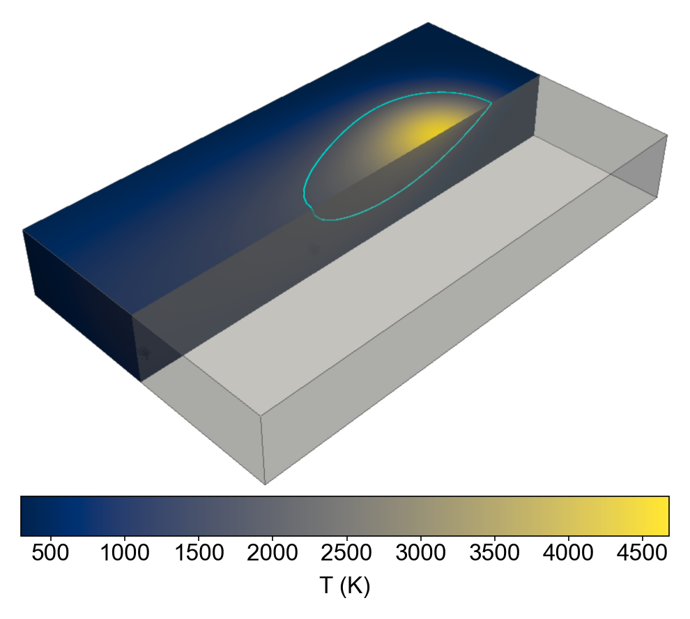
plot_temperature_field_3d computes the full (nx, ny, nz) temperature array and renders it as a volumetric visualization using PyVista.

By default the function returns a matplotlib.Figure from an off-screen render, making it suitable for saving figures in non-interactive environments. Pass return_plotter=True to get the live pyvista.Plotter object for interactive exploration.

from eagar_tsai import BeamParameters, MaterialProperties, SimulationDomain
from eagar_tsai.plot import plot_temperature_field_3d

beam = BeamParameters(
    beam_diameter=100e-6,
    power=200.0,
    velocity=0.5,
    absorptivity=0.35,
)

material = MaterialProperties(
    liquidus_temperature=1700.0,
    thermal_conductivity=30.0,
    density=7800.0,
    specific_heat=700.0,
)

domain = SimulationDomain(
    x_length_um=450.0,
    y_length_um=180.0,
    z_depth_um=80.0,
    spatial_resolution_um=10.0,
)

# Off-screen render — returns a matplotlib Figure
fig = plot_temperature_field_3d(beam, material, domain, workers=-1)
fig.savefig("temperature_volume.png", dpi=300, bbox_inches="tight")

# Interactive window
plotter = plot_temperature_field_3d(beam, material, domain, workers=-1, return_plotter=True)
plotter.show()

The mirror_y option (default True) reflects the half-domain computation to display the full symmetric melt pool. The liquidus_contour option (default True) overlays the liquidus isotherm as a contour surface. Passing output_vti saves the volume to a .vti file for use in ParaView or other VTK-compatible tools.

3D temperature volume for 316L stainless steel (T_liq = 1700 K, k = 30 W/(m·K), ρ = 7800 kg/m³, c_p = 700 J/(kg·K)). Beam conditions: P = 200 W, v = 0.5 m/s, d = 100 µm, A = 0.35. The liquidus isotherm contour marks the melt pool boundary.

Printability Maps

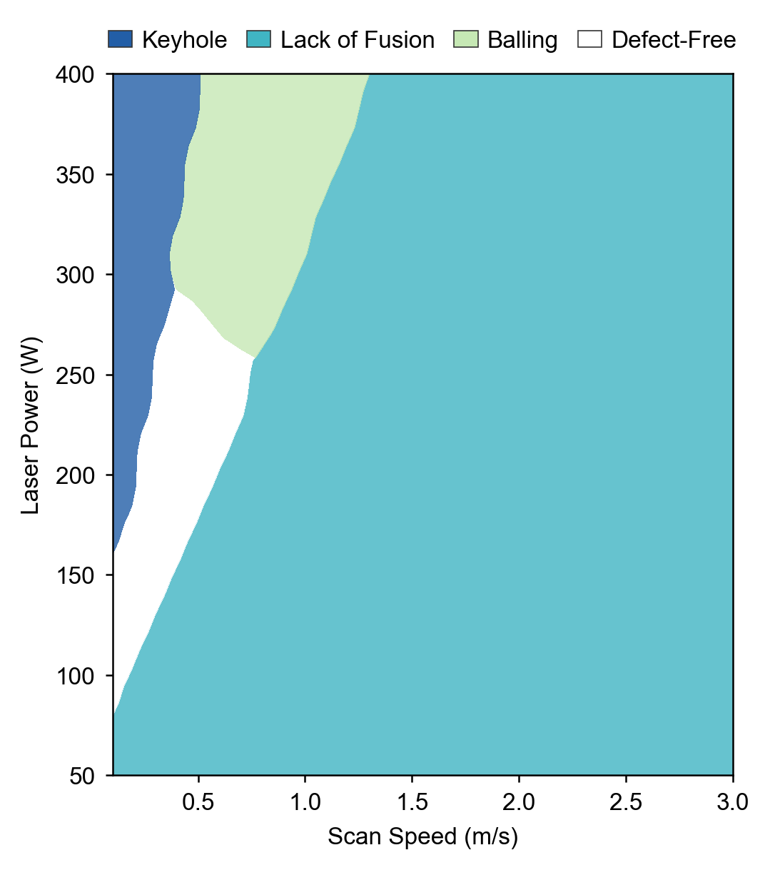
compute_printability_map sweeps laser power and scan speed over a regular grid, runs the Eagar–Tsai model at every grid point, and classifies each point into one of four defect regimes (keyhole porosity, lack of fusion, balling, or defect-free).

Parallelism

Each grid point is dispatched as an independent task to the worker pool. Workers stay fully utilized even when isolated points require iterative domain expansion.

The fixed process parameters (beam diameter, absorptivity, layer thickness, hatch spacing) are specified through a PrintabilityParameters object:

from eagar_tsai import (
    MaterialProperties,
    PrintabilityParameters,
    SimulationDomain,
    compute_printability_map,
)

material = MaterialProperties(
    liquidus_temperature=1700.0,   # K
    thermal_conductivity=30.0,     # W/(m·K)
    density=7800.0,                # kg/m³
    specific_heat=700.0,           # J/(kg·K)
)

process = PrintabilityParameters(
    beam_diameter_m=80e-6,         # m
    absorptivity=0.35,
    layer_thickness_m=40e-6,       # m
    hatch_spacing_m=90e-6,         # m
)

# 5 µm resolution domain, fast per-point computation
domain = SimulationDomain(
    x_length_um=1200.0,
    y_length_um=1200.0,
    z_depth_um=1000.0,
    spatial_resolution_um=5.0,
)

df = compute_printability_map(
    process,
    material,
    power_range=(50.0, 400.0),    # W
    velocity_range=(0.1, 3.0),    # m/s
    n_power=50,
    n_velocity=50,
    domain=domain,
    workers=-1,                    # use all CPU cores
)

print(df["defect"].value_counts())

The returned DataFrame has one row per grid point with columns power_w, velocity_m_s, melt_length_um, melt_width_um, melt_depth_um, defect, and one boolean flag per criterion (lof1, lof2, ball1, ball2, kh1).

plot_printability_map wraps compute_printability_map and renders the result directly:

from eagar_tsai.plot import plot_printability_map

fig = plot_printability_map(
    process,
    material,
    power_range=(50.0, 400.0),
    velocity_range=(0.1, 3.0),
    n_power=50,
    n_velocity=50,
    domain=domain,
    workers=-1,
    output="printability_map.png",
)

Printability map for 316L stainless steel (T_liq = 1700 K, k = 30 W/(m·K), ρ = 7800 kg/m³, c_p = 700 J/(kg·K)). Process parameters: d = 80 µm, A = 0.35, layer thickness = 40 µm, hatch spacing = 70 µm. Grid: 40 × 40 points over P = 50–400 W and v = 0.1–3.0 m/s. Regions are classified as keyhole porosity, lack of fusion, balling, or defect-free.

Parallel Processing

workers sets the number of parallel processes (-1 uses all CPU cores); chunk_size controls how many rows each worker receives at a time.

# Use all available CPU cores
result = compute_melt_pool(df, workers=-1)

# Use 8 workers, process 50 rows per chunk
result = compute_melt_pool(df, workers=8, chunk_size=50)

Note

Setting workers=None or workers=1 runs serially in the current process. This is recommended for small datasets or debugging.

Saving Intermediate Results

When output_dir is set, each completed chunk is written to a numbered CSV file (ET_0000.csv, ET_0001.csv, …) immediately, so results are preserved if the run is interrupted.

from pathlib import Path

result = compute_melt_pool(
    df,
    workers=4,
    chunk_size=50,
    output_dir=Path("calc_files"),  # saves ET_0000.csv, ET_0001.csv, ...
)